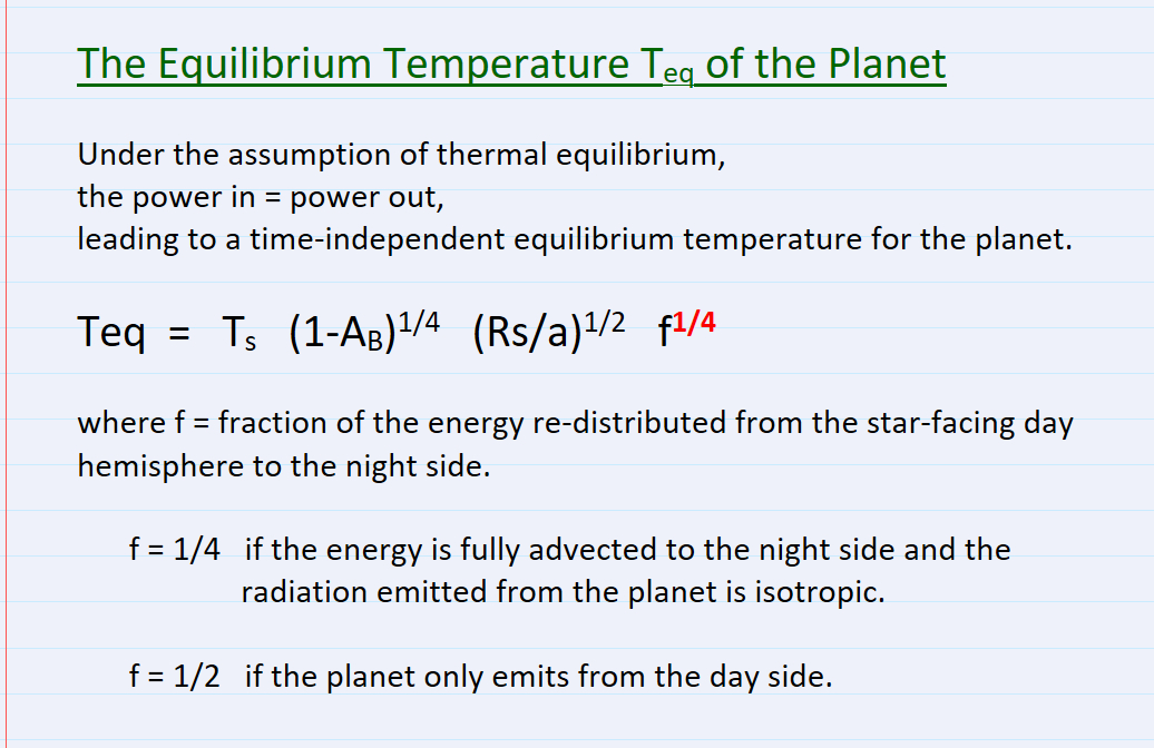
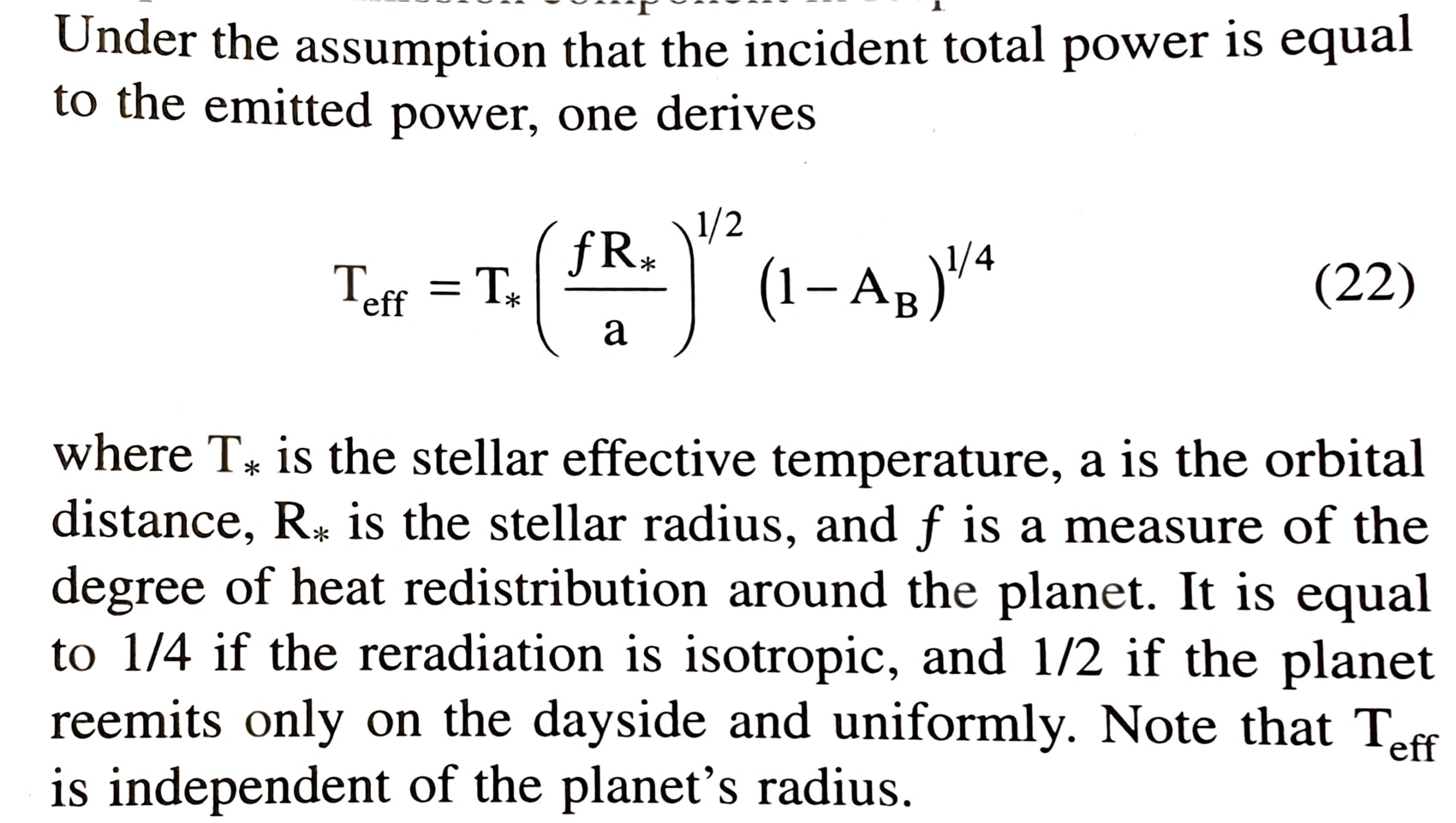
ERRATUM: For our Lecture 21 (corresponding to the old 2021 Lecture 23 notes on Canvas), there were a pair of typos in the exponents. Here is the correction:

ERRATUM: For our Lecture 21 (corresponding to the old 2021 Lecture 23 notes on Canvas),
there were a pair of typos in the exponents. Here is the correction:
May 3:
- Read Haswell Chapter 7
- "Lightly" Read Perryman Chapter 10.0-10.2; 10.10
- "Lightly" Read Perryman Chapter 11.0-11.2; 11.4-11.41; 11.5, 11.6, 11.7.
* Study for Final Exam on Monday May 10th, 1:00-3:00 pm
April 17: Homework #14
* MLO remote observing from PA-215 on on Thur, or Fri, or Sat nights, from 7pm-midnight
- Review CCD Calibration notes.
- Install AstroImage J (AIJ).
- Read / review the AIJ Flash Guide and User Guide.
- Study for Exam #2 on Monday April 24.
Journal Reading Homework:
- - Read the paper on the discovery of ellipsoidal variations of HAT-P-7 and the
associated notes.
Apr 10: Homework #13
- Continue refining your presentation for Wednesday April 12. Send me your title.
- Read Haswell's Chapter 6.
Written Homework #13: (due Monday April 17)
1. Do Exercise 3.4 (page 102) in Haswell's book -and- also plot the three limb
darkening laws. In other words, plot the relative intensity I/I0 vs.
mu. As always, comment on the results.
2. Show that a planet's surface gravity "g" can be expressed in terms of
observables from RV and transit data, and do NOT depend on knowing the mass
or radius of the host star (i.e., derive equation 4.49 in Haswell's book).
Apr 3: Homework #12
* Exam #2 postponed until Monday April 24 *
- Continue working on your class presentation (due April 12).
- Review the class notes on CCD data calibration.
- In Haswell's book, read Chapter 4 and the rest of Chapter 5 (you already read Sec 5.3).
(Chapter 5 is the more important of the two chapters; you can "lightly" read
Chapter 4).
- "Lightly" read Chapter 7 in Perryman's book. In particular, focus on sections
7.0-7.41 and 7.9-7.10
- [Highly recommended, but not required reading]: The excellent and thorough chapter
by Josh Winn called "Transits and Occultations" in the "Exoplanet" book edited by
Sara Seager (Univ. Arizona Press).]
Mar 20: Homework 11
- Write up your presentation topic and submit this as written homework
assignment #10, due WEDNESDAY March 22.
* Exam #2 postponed until ... *
- Read Chapter 3 in Haswell's book.
- Continue/finish reading Chapter 6 in Perryman's book (from the start now).
- Continue working on your class presentation (due April 12).
- Review the class notes on CCD data calibration and differential aperture photometry.
- Read the AstroImageJ (AIJ) "Flash Guide" and start the process of getting
AIJ installed on a computer that you can use to calibrate and fit data.
Written Homework #11: (due Wed April 5th)
1a. Determine which transiting exoplanets can be observed from
MLO on April 20-22 (civil nights Thurs, Fri, Sat).
From your list of targets, find those for which
(i) transit depth is at least 1 percent;
(ii) mid-transit occurs in the early part of the evening, ideally 8:00-10:00 pm,
but slightly outside this range is okay.
1b. Choose one target you prefer to observe, and explain why.
To do this assignment, it is necessary to use an ephemeris tool. Two that
I can recommend are (i) "skycalc" by John Thorstensen and its more modern
image/GUI-driven Java version called "JSkyCalc"; and
(ii) the NExSci Exoplanet Archive website.
There are probably many other similar tools available.
Mar 5: Homework 10
- Study for Exam #1 on Wed March 15.
- Work on your Presentation topic, due Monday, March 20th.
A title and half-page description of the topic is sufficient.
Include at least 3 references for now (many more needed later).
Explain what the topic is about, why it is important (the motivation),
and what you will cover in your 5-min presentation on Wed April 12th.
See the "Presentation" section of the syllabus on page 2 for more info.
Journal Reading Homework: The Radial Velocity Method Part 3
- Hubble Space Telescope Time-Series Photometry of the Transiting Planet HD 209458
by Tim Brown, Dave Charbonneau, Ron Gilliland, Bob Noyes, and Adam Burrows
(2001 ApJ 552, 699). [This is the famous paper that
kick-started the field of high-precision transit science. In my opinion, this is
the second most important exoplanet paper ever published, after the 51 Peg paper
by Mayor and Queloz.]
- System Parameters of the Transiting Extrasolar planet HD 209458b
by Rob Wittenmyer et al. (2005). [Rob was an SDSU grad student and most of this
work was in his MS Thesis.]
Mar 1: Homework #9
- In Haswell's book, read Chapter 4 and 5, with emphasis in Ch 5.3
(the Rossiter effect). You can start with Ch 5.3, then go back and read
sequentially from the start of Ch 4.
- In Perryman's book, read Chapter 6.18
Journal Reading Homework: The Rossiter Effect:
- "The Rossiter-McLaughlin effect for exoplanets" by Josh Winn
- "Planets in Spin-Orbit Misalignments and the Search for
Stellar Companions" by Brett Addison, et al.
Note: I suggest reading Ch 5.3 in Haswell's book (and possibly Ch 6.18
in Perryman) before reading the above papers.
- Begin studying for Exam 1.
The focus will be on the material covered in class, Haswell's Ch 1, 2, 4, 5.3,
Perryman's Ch 1, 2, 6.18, the papers assigned for homework, and the homework
exercises.
Feb 22: Homework #8
Written Homework #8, due Wed March 1.
Use the Systemic Console tool to make RV fits to
51 Peg and also HD 17156
(use the data on the Systemic Console pull-down menu).
Turn in the Systemic Console figures and/or screencaptures.
Comment on your results.
Feb 20: Homework #7
- In Perryman's book, review Chapters 1 and 2.
Journal Reading Homework: The Radial Velocity Method Part 2
- "Doppler spectroscopy as a path to the detection of Earth-like planets"
by Mayor, Lovis & Santos (2014 Nature Review article)
- "On the Determination of Transiting Planet Properties from Light and Radial
Velocity Curves" by John Southworth (2017 PASP)
Use Gregg Laughlin's Systemic Console tool to play with and fit
radial velocity data. It used to be hosted on Laughlin's fascinating
oklo blog but that link is gone (and the
blog is less and less about planets in the past few years - but the archive
is magnificent). So you can get to Systemic
from Stephano M. who maintains (or used to maintain) a version of
Systemic 2 and Systemic Live.
Feb 13: Homework #6
Reading homework:
- In Perryman's book, continue reading about the RV method (Chapter 2).
Journal Reading: The Radial Velocity Method Part 1
- Read the famous 51 Peg discovery paper by Mayor & Queloz (1995). This is
the paper that kickstarted the modern field of exoplanet astronomy, and
helped earned the authors the Nobel Prize.
Written Homework #6, due Wednesday Feb 22:
1. Take the white noise and red noise data sets that your created for
Homework #5 Part 3 and cut them into pieces to give you the first quarter,
the first half, and the whole thing (no cut). Compute the mean and
standard deviation (or rms) for the three parts. What do you notice
for the white versus the red noise? Comment on the results.
2. Use the NExScI Exoplanet Archive periodogram tool to make periodograms
and phase-folded plot of the four fake data sets that you created for
Written Homework #5 part 3. Turn in the NExSci figures and/or screen captures.
Comment on the results.
3. Repeat the above, but use xmgrace (called "qtgrace" under Windows) or
some other software tool/package to make power spectra (not periodograms).
Comment on the results.
4. Explore - play - learn - have fun!. Create new data sets and see what
their power spectra look like. Develop some intuition.
Part 4 will not be graded, and you do not need to turn anything in.
But arguably this is the most important part of the homework.
If you do submit an answer I will read and comment on it, but it won't
affect your grade.
Feb 6: Homework #5
- Explore the NASA Exoplanet Archive. See what data sets and (especially)
what tools are available.
- Journal Reading: Evryscope:
"Evryscope Science: Exploring the Potential of All-Sky Gigapixel-Scale
Telescopes" (Law et al. 2015 PASP 127, 234)
See also the Evryscope Poster paper by Nick Law, et al.,
presented at the Keele Transiting Exoplanets conference (2017 July 17-21).
- Written Homework #5, due Wednesday Feb 15:
1. Haswell Exercise 1.4, page 33, Part (c) only. Show all work.
2. What is the amplitude of the Sun's RV reflex motion due to the Earth?
3. Write some code to generate artificial light curves that (separately)
exhibit these three phenomena: (a) sinusoidal (b) white noise (c) red noise.
Then create a light curve with (d) all three of these features combined,
with roughly the same amount of RMS power. Describe how you generated the time
series (but I don't want to see any code) and turn in the figures.
Be sure to label all axes and have smart-looking plots like you would see
in a journal (e.g. don't have a ton of wasted white space on the figure).
Choose sensible units.
Comment on your results.
Feb 1: Homework #4
Reading Homework:
- In Perryman's book, continue reading Chapter 2.
Journal Reading: M-star Planet Searches:
- "Design Considerations for a Ground-Based Transit Search for
Habitable Planets Orbiting M Dwarfs", Nutzman & Charbonneau
2008 PASP 120, 317
- "A super-Earth transiting a nearby low-mass star"
Charbonneau, et al. Nature, 462, Issue 7275, pp. 891-894 (2009)
Written Homework #4, due Wednesday Feb 8:
1. What are the advantages are of searching for planets around M-stars?
What are the disadvantages?
2. What does the term "astrophysical false positive" mean in the context
of exoplanet searches?
As always, comment on your answers/results.
* Note: Next week's assignment will require some very simple programming to
generate artificial data sets (sine waves, etc., and compute their RMS power).
If you are not (yet) comfortable with programming, please see me for some
help well before this assignment is due..
Jan 30: Homework #3
* Be sure you are comfortable plotting things. I recommend xmgrace
if you don't already know how to quickly make quality figures.
(NB: xmgrace is called "qtgrace" under the Windows OS and some Mac OS
versions.)
Reading Homework:
- In Perryman's book, start reading Chapter 2.
Journal Homework: Ground-based Planet Searches Part 2:
- "The WASP Project and the SuperWASP Cameras", Pollacco, D. et al. 2006
PASP, 118, 1407
- "The Kilodegree Extremely Little Telescope (KELT): A Small Robotic
Telescope for Large-Area Synoptic Surveys", Pepper, J. et al.
2007 PASP 119, 923
Jan 23: Homework #2
Thinking Homework:
(I will not be collecting or grading this assignment.)
Suppose you are working on your mission to find exoplanets, and you have
decided to embark upon a wide-field transit survey. You have big pixels
on the sky. Why would you want to purposely degrade the image quality of the
seeing? Despite worse crowding, and more sky noise, how/why would a bigger
PSF actually help? Try answering this question without looking up any papers -
just think about what's going on.
It is very important that you attempt to answer this before reading the
article by Gaspar Bakos about the HATnet. Then, after you have read the
paper, go back and update your answer. If you want to change your thoughts,
do so by appending a correction. It is important that you do not delete
anything in your original answer. Don't delete or cross out your original
answer, simply add more to it.
Written Homework #2, due Wed Feb 1:
Make a list of the on-sky pixel size (i.e. arcsec/pix) for the various
transit-search programs (HAT, WASP/SuperWASP, KELT, MEarth, Kepler,
TESS, etc.). Also, find (or calculate) the pixel scale for the MLO
40-inch telescope. In addition, it would be good to pick other
telescopes, not designed for transit searches and see what the pixel
scale is for those (e.g. MLO's Evryscope, HST, JWST, etc.). Then, comment
on what you find.
Reading Homework:
- In Haswell's book read Chapter 2.
- In Perryman's book read Chapter 6.1-6.5 (pages 153-171)
Journal Reading: Ground-based Planet Searches Part 1
- "Wide Field Millimagnitude Photometry with the HAT: A Tool for
Extrasolar Planet Detection", Bakos et al., 2004 PASP 116, 266
Jan 18: Homework #1
Reading Homework:
- Read the syllabus carefully, read the class policies on the class website.
- Explore some of the links on the class website.
- In Haswell's book, start reading Chapter 1
- In Perryman's book, begin reading Chapter 1
Written Homework #1, due Wed Jan 25:
Although I wont collect this homework, please do write down your thoughts.
1. Generate a few questions from your reading of Chapter 1 in each book.
We will discuss/answer some of these questions in class.
2. Suppose you are in charge of an observatory and want to find planets via
the transit method. What things do you need to consider?
![]()
Homework Philosophy & Grading Policy:
The homework assignments (15% of the course grade) are designed to be
relatively easy and broad in scope. They are really a warm-up to get you
thinking. Consequently,
Each homework is worth 50 points.
Late Homework Policy:
Late homework will incur a penalty as follows:
- 4 points deducted for 1 day late; 1 point deducted each day thereafter.
The maximum penalty is 10 points (after 1 week). In other words, there
is a floor beyond which no additional loss of points will occur. Even if
you are 3 weeks late in doing the assignment, it is much better than not
doing it at all. The only exception is if the answer to the homework
question is discussed in class, in which case that problem is no longer valid
for late credit; late homework earns zero credit for this problem.
If a student is observing the night before a homework is due, the student
can take 1 extra day to hand in the homework without penalty,
**with permission in advance.**
If a student is defending their thesis (dissertation or paper) within +/- 2
days a homework, paper, or presentation is due, the student can get a few
extra days of time without penalty, **but only with permission well in
advanced.**